posts > stats
Time Complexity for Data Scientists

This article has been published in Towards Data Science
Big data is hard, and the challenges of big data manifest in both inference and computation. As we move towards more fine-grain and personalized inferences, we are faced with the general challenge of producing timely, trustable, and transparent inference and decision-making at the individual level [1]. For now, we will concern ourselves with the challenge of “timeliness”, and try to gain intuitions on how certain algorithms scale and whether or not they can be feasibly used to tackle massive data sets.
In inference, there is never “enough” data. As you get more and more data, you can start subdividing the data to gain better insights among groups such as age groups, genders, or socio-economic classes [2].
N is never enough because if it were “enough” you’d already be on to the next problem for which you need more data. — Andrew Gelman
This insatiable need for data gives rise to challenges in computation (and cost). Some of these problems can be addressed with “brute-ish force” using a lot of computing resources through parallelization. Other problems are simply computationally intractable without the proper approach.
Simply put, the size of the data puts a physical constraint on what algorithms and methods we can use. So as data scientists and problem solvers, it is important that we are conscious of how our certain models, algorithms and data structures work and how they perform at scale. This means that we should have familiarity with what tools we have available and when to use them.
What to expect
This is a pretty long post with 4 parts. In parts 1 and 2, I try to give an in-depth (and hopefully intuitive )introduction to algorithms and time complexity. If you are fairly familiar with time complexity then you can skip to parts 3 and 4.
- Getting started with time complexity: what is time complexity, how does it affect me, and how do I think about it?
- From slow to fast algorithms: What makes an algorithm fast? How can two solutions for the same problem have radically different speeds?
- Basic Operations: How fast/slow are some of the routine things I do?
- Problems with Pairwise Distances: How do I find the nearest neighbors quickly? How do I find similar and near-duplicate documents quickly? How fast are my clustering algorithms?
Getting started with time complexity

Let’s start with a leisure stroll through some examples to give you an idea of how to think about algorithms and time complexity. If you are fairly familiar with time complexity you can skip this section.
Intersection of two lists
A few years ago, one of my workmates was tasked to get descriptive statistics on their platform’s frequent customers. He started by getting a list of the current month’s customers and comparing it with the previous month’s customers. He had two python lists curr_cust and prev_cust, and his code looked something like:
common_cust = 0
for cust in `curr_cust`:
    if cust in `prev_cust`:
        common_cust += 1
He started with a sample list of around 4000 customers for each month and this code snippet ran for around 30 seconds. When this was used with the full list of around 3 million customers, these few lines of code seemed to run forever.
Is it because Python is just slow? Should we move to C/Go to optimize? Do we need to use distributed computing for this? The answer is no. This is a very simple problem and the fix is even simpler, which can run in around 1 second.
common_cust = 0
prev_cust_set = set(prev_cust)
for cust in curr_cust:
    if cust in prev_cust_set:
        common_cust += 1
For people with a background in computer science or programming in general, this fix should be fairly obvious. But it is understandable how people coming from backgrounds with less emphasis in computation might see little difference between the two code snippets above.
Briefly, the difference boils down to the difference between a python list and set . A set is designed to do these "is this element in" operations quickly. Even if you double the number of elements inside **prev_cust_set** the operation **cust in prev_cust_set** will take about just as long.
On the other hand, if you double the size of a **prev_cust**, the operation **cust in prev_cust** would take twice as long to run. If you are wondering how the set does this, it uses hashes with a data structure like the hash table/set, which can also be implemented with some version of a binary search tree.
Time complexity and the big O
We know there is a difference between the code snippets, but how do we express this difference? This is where the big O notation comes in.
Although there are formal definitions of big O, you can mainly think of this as an estimate for the number of “operations” that a machine does to finish the algorithm. The number of operations strongly relates to the “running time”, and it is often parameterized with the size of the data. You might hear something like, “The classic SVD decomposition has cubic complexity.” and something you might encounter in the documentation of the algorithms you are using.
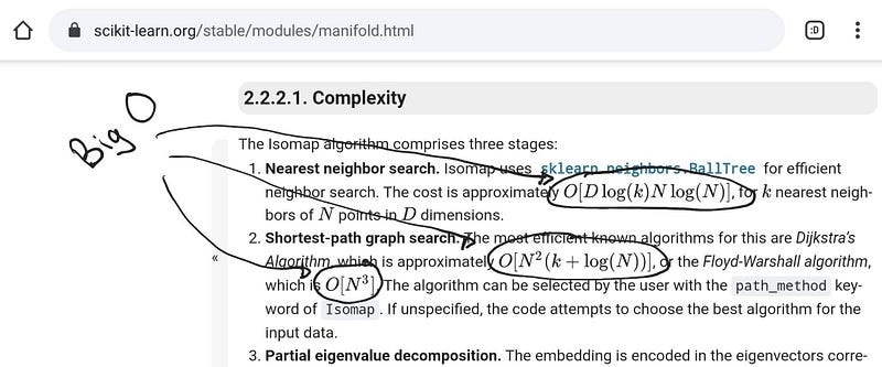 Big O’s in scikit-learn’s documentation
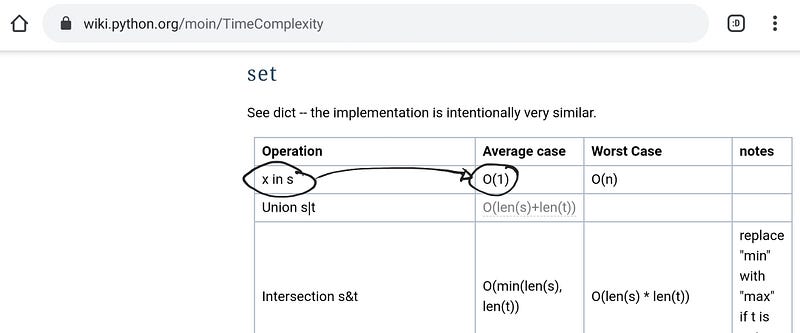
And if we look in the python’s documentation on Time Complexity, we can read that for operations that have the form x in s :
- O(n) if
sis alist - O(1) if
sis aset
Let’s start with the list example to see that it is O(n²), where n is the number of customers per month.
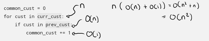
The general steps are:
- We loop through each customer in
curr_cust, and there arencustomers - For each customer
cust, we check whether or not it is in listprev_cust. According to the docs, this is O(n), but intuitively, to do this, we potentially need to check every customer inprev_custto see whether or notcustis one of them. There arencustomers inprev_custso this takes at mostnoperations - Adding a number is just 1 step.
Each iteration of the loop takes around O(n) + O(1) steps, and there are n iterations in the loop, so putting all that n(O(n) + O(1)) = O(n²).
You can add and multiply O’s together and when you have several terms, you just drop the lower ordered terms and drop coefficients. O(n²+n) = O(n²).
We can do the same thing for the code using set , the only difference is that cust in prev_cust_set runs in O(1) time (on average).
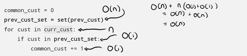
The general steps are:
- There’s a preprocessing stop to create the set. Let’s just take this as O(n)
- We loop through each customer in
curr_cust, and there arencustomers - For each customer
cust, we check whether or not it is in listprev_cust_set. This takes O(1) - Adding a number is just 1 step.
Putting it all together: O(n) + n(O(1) + O(1)) = O(2n) = O(n). Compared to the list implementation, the set is blazingly fast.
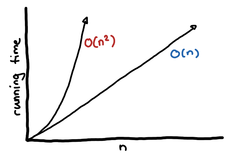
Interpreting big O
So we have one algorithm that is O(n²) and another algorithm that is O(n). How do you interpret this?
One way of looking at this is getting an estimate of the magnitude of the problem by plugging in the estimated value of your data set, n. If the size of our data is 3 million then there would be around 3000000² operations for an O(n²) algorithm, which is around 9000000000000, which is a lot.
The same data set but using the O(n) algorithm would have around 3000000 operations, which is much more manageable.
Recall that we drop lower order terms and coefficients when we compute the big O. So the exact value isn’t important here. We look only at the magnitude of the problems. A million operation algorithm is much better than a ten trillion operation algorithm.
Another way of looking at this is by getting the relative ratio between two data set sizes. This is useful if have empirical benchmarks of each of the algorithm and want to extrapolate when scaling up.
So let’s say that at 40000 customers, the list algorithm took 30 seconds. If we double the size of the data how long would it take? So we now have a dataset that has a size of 2n. Then the running time would be around
O((2n)²) = O(4n²)
This means doubling the size of the dataset for an O(n²) would increase the running time by a factor of 4. We expect it to run for around 120 seconds.
On the other hand, for the set algorithm is equal to O(2n) which means that doubling the data set only doubles the running time.
The big difference in performance comes from the subtle difference between cust in prev_cust and cust in prev_cust_set. These kinds of differences are a bit harder to notice when a lot of the code that we use are abstracted from us in the modules that we use.
The big O notation gives us a way to summarize our insights on how the two algorithms above scale. We can compare O(n²) vs O(n) without knowing exactly how each algorithm is implemented. This is exactly what we did when we used the fact that x in prev_cust_set is O(1) without describing how exactly the set implements this. What big O gives us is a way to abstract the algorithm by describing the general shape that the running time has with respect to the input size.
Being aware of these differences can help us gauge whether or not a particular approach with a small sample of the data will scale when done in production. What you do not want to happen to you is to do an experiment or POC on a small sample, present good results and get a go signal from the stakeholders, only to find out that your algorithms cannot handle all the data.
On the other hand, if you know that the data sets are not massive, then you can opt to use slower algorithms and models that either give better results or are much simpler to implement and maintain.
From slow to fast algorithms

Before we start our trek to explore the time complexities of the different tools and techniques that we use in data science, I’ll start by going through methods of solving a much simpler problem, the range query problem. For each algorithm, we discuss briefly how it works and its consequent properties. Hopefully, after going through this progression of algorithms, you will get a better feel of algorithms and time complexities.
Range query problem
Assume that we have an array of numbers of size N.
arr = [443, 53, 8080, 420, 1989, 42, 1337, 8008]
In the example above, the index starts at 0:
arr[0] = 443arr[1] = 53arr[4] = 1989
You are tasked to get the sum of all numbers between index a and b for some query query(a, b).
Let’s say that the query is query(2, 5) . Then the answer should be 10531
arr[2] + arr[3] + arr[4] + arr[5]
8080 + 420 + 1989 + 42
10531
Another possibly optional operation is updating an element in the array, update(idx, new_val)
update(3, 88)
query(2, 5)

# arr[2] + arr[3] + arr[4] + arr[5]
# 88 + 420 + 1989 + 42
# 3539
Naive Solution
The simplest solution is to just loop through the list and get the sum.
def query(a, b):
    return sum(arr[a: b+1])
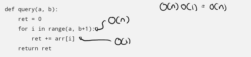
Although the code above has very few code, it is actually doing a lot of things already. For clarity, we will unpack sum(arr[a: b+1]) to the following query:
def query(a, b):
    ret = 0
    for i in range(a, b+1):
        ret += arr[i]
    return ret
The total complexity of query(.) is based on how many elements are in the queried range. This depends on a and b, with the total number of elements summed as b — a + 1 , and when dealing with the big O notation, we look at the worst case of this value, which this can reach up to N when querying the sum of the entire array.
To update the array, we simply update the element on that particular index:
def update(idx, new_val):
   arr[idx] = new_va
This update(.) function obviously runs in O(1) time, or in constant time. No matter how big the array is, this function runs the same number of operations.
For the naive solution, we have the following time complexities:
- query: O(N)
- update: O(1)
The problem with this is if the array is queried a lot of times, then for each query, you have an O(N) operation. For q queries, you will have a total of O(qN) solution.
Is this acceptable? It depends. If you have a large array and a lot of queries, then no this is not acceptable. Think about when you have around 1,000 queries for a 1,000,000 sized array.
If the data is small, then problems like this become trivial.
Prefix Sum
To address the shortcomings of the naive solution, we introduce using a prefix sum. We transform the original array so that queries are faster.
The prefix some arr_sum is an array where the value at a particular index is the sum of all elements up to that index in the original array.
arr = [443, 53, 8080, 420, 1989, 42, 1337, 8008]

arr_sum[0] = 0
arr_sum[1] = arr[0]
arr_sum[2] = arr[0] + arr[1]
arr_sum[3] = arr[0] + arr[1] + arr[2]
...
arr_sum[8] = arr[0] + arr[1] + arr[2] ... + arr[7]
However, this particular construction of the prefix sums is slow. To construct arr_sum takes O(N²) time, since there are N cells in arr_sum to be filled up each one with summing up to N elements of arr .
We can construct arr_sum more efficiently by noting that only difference between arr_sum[3] and arr_sum[2] is arr[2]
arr_sum[2] = arr[0] + arr[1]
arr_sum[3] = arr[0] + arr[1] + arr[2]
arr_sum[3] = arr_sum[2] + arr[2]
So a better construction for arr_sum is as follows
arr_sum[0] = 0
arr_sum[1] = arr_sum[0] + arr[0]
arr_sum[2] = arr_sum[1] + arr[1]
arr_sum[3] = arr_sum[2] + arr[2]
...
arr_sum[8] = arr_sum[7] + arr[7]
This takes O(N) time since there are still N cells, but each cell only needs 2 values to be computed. If done correctly arr_sum would result to:
arr_sum = [0, 443, 496, 8576, 8996, 10985, 11027, 12364, 20372]
Now how do we use this? If we have a query for 2 and 5 then we can use the prefix sum from 0 to 5 and subtract from it the prefix sum from 0 to 1 to get the sum from 2 to 5.
def query(a, b):
    return arr_sum[b+1] - arr_sum[a]
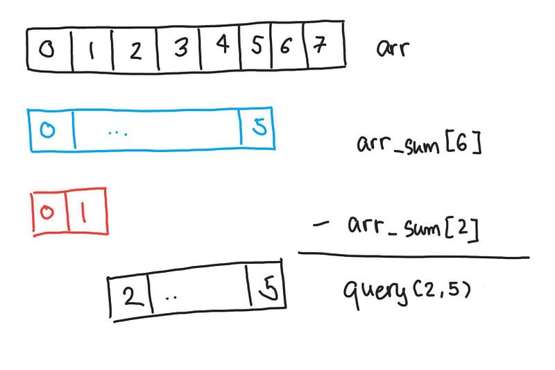 Getting the sum of index 2 to 5
In a way, we have a cache of the answers for any query. We are precomputing some values that help us in the queries. It should be clear that no matter how large the range of query(a, b) the function only needs to look up 2 values, so the querying time is constant, O(1).
What if the update operation is needed? Then updated a single element will mean than all prefix sums that contain that element needs to be updated as well. This can mean that we might need to reconstruct the prefix sum, which runs in O(N) time.
For the prefix sum algorithm, we have the following time complexities:
- query: O(1)
- update: O(N)
We see this trade-off between optimizing queries and updates. If we optimize queries, then it requires us to maintain a data structure (the prefix sum array we have is a data structure) and this has overhead when it comes to updating elements of the original array. However, we do not want to maintain the data structure, then each query requires us to go through every element in the queried range.
Segment Trees
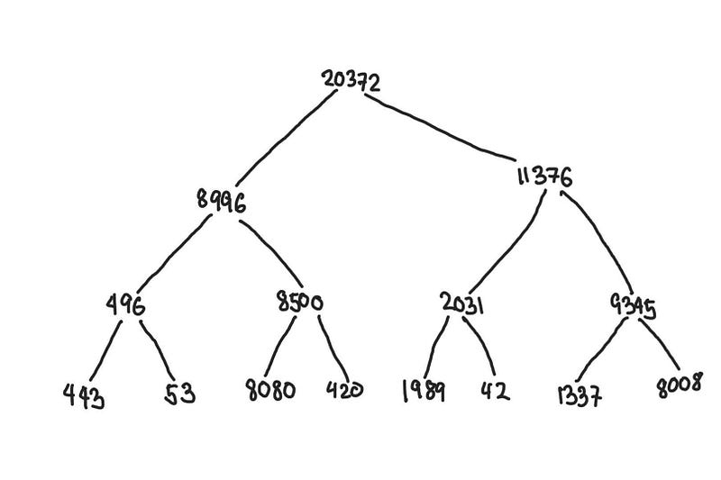
A particular data structure that we construct that is able to balance between queries and updates is a segment tree. This is a binary tree where each node represents a segment.
In the illustration below, we have a segment tree constructed from arr . The leaf nodes at the bottom are the elements of the original array, and each node’s value is just the sum of its children.
arr = [443, 53, 8080, 420, 1989, 42, 1337, 8008]
 Segment tree constructed from arr
We relabel the tree above to highlight what segments each node represents. The topmost node contains the sum of the entire array from index 0 to 7.
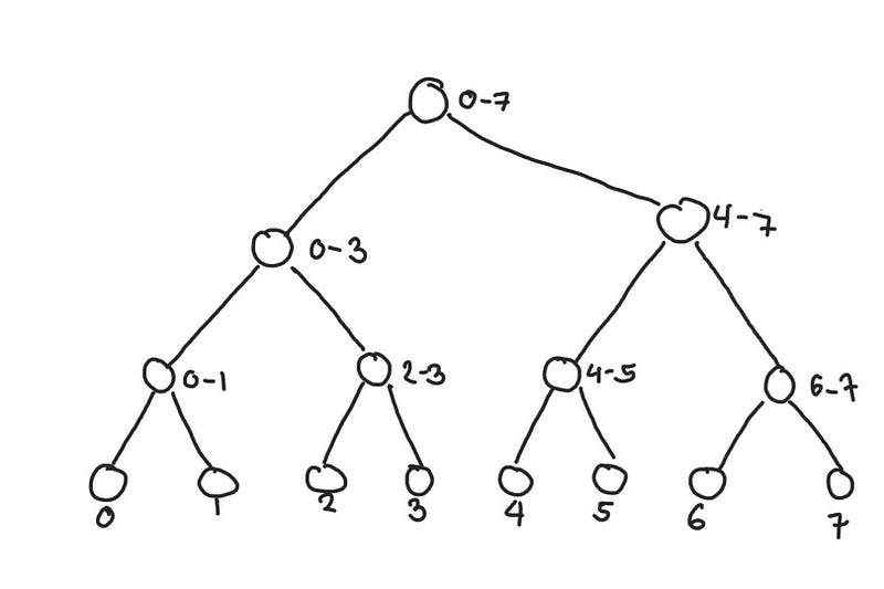 The number beside the node represents the range of indices of the segment it represents
So how do we make query from this? The concept is similar to the prefix sum where we can use segments of the array that we have precomputed to compute the queried range. The difference here is that the segment tree is more flexible in the segments it can represent.
Let’s say we want to find query(2, 5) . Getting the sum of the highlighted nodes would result in the correct answer. Although the proof isn’t as straightforward, but the number of nodes you need to access is naturally very small compared to the actual size of the ranges of original array. This operation takes O(log n) time.
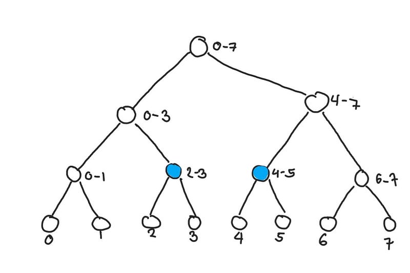 Getting the sum from elements 2 to 5
Here is another example of a query. Let say we query(3, 7)
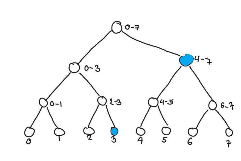 Getting the sum from elements 3 to 5
Because of the way the segment tree is made, when we update a leaf node, the only nodes that need to be updated are the nodes between the leaf node and the root node. Below we see what nodes need to be updated if we update the element at 5. This operation also takes O(log n) time, since each node up the tree doubles the size of the represented segment.
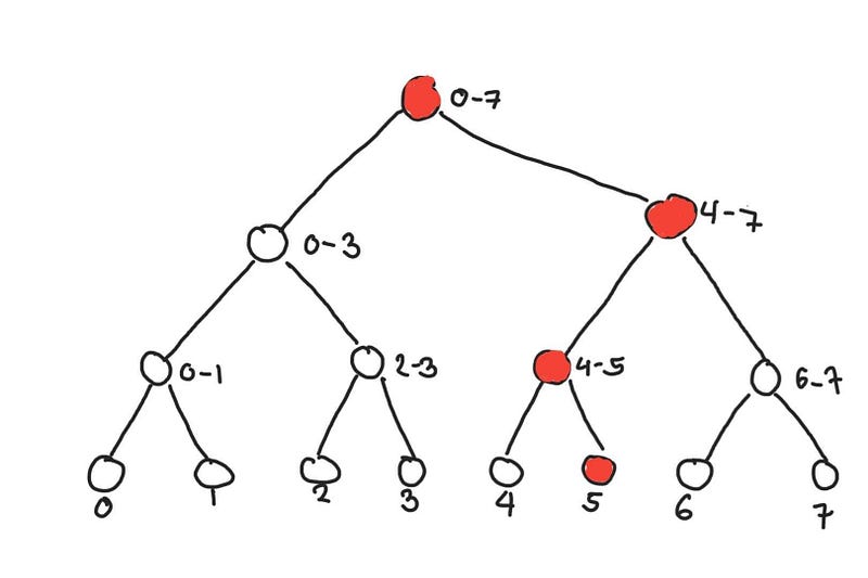 Nodes that need to be updated when updated element 5
For the segment tree data structure, we have the following time complexities:
- query: O(log n)
- update: O(log n)
With a more sophisticated data structure, we are able to balance the trade-off between queries and updates. However, this data structure is a lot more complicated to implement that your naive or prefix sum algorithms. The exact implementation of the segment tree will not be discussed here.
Note: A usual algorithm that is usually discussed before the segment tree is the Fenwick Tree. Although Fenwick tree is easier to implement, I feel the segment tree is much more intuitive. So I opted to skip discussing that.
Even faster algorithms?
As you can see, the way we approach the problem can dramatically change the performance of our algorithms (from a quadratic to log-linear performance). This can come in doing some clever preprocessing, finding a way to representing the data more efficiently, or using some properties of the data.
A way to mitigate this is to throw more computational resources. However, some algorithms that we have were designed in a time where you had this single powerful machine. These may not lend themselves to parallelization.
However, there are some problems where finding faster algorithms can be very difficult, and the fastest algorithms are still not fast enough. In such cases, one approach to find faster solutions is by relaxing the problem. The solutions discussed above give exact solutions, but there are times where we don’t need the best answer. What we need are good enough answers.
We can do this through one of several ways:
- solve for an approximate solution (from shortest path to shortest-ish path, or k-_nearest neighbors_ to k-near-enough neighbors)
- use algorithms that use probabilistic processes where you will probably get the right answer most of the time (Locality Sensitive Hashing and Approximate Cardinality)
- use an iterative approach that converges (Stochastic Gradient Descent or Power iteration)
- use algorithms that perform well on the average case (KD-Trees)
- (re)design algorithms to be parallelizable
We will encounter some of these when we go through the different algorithms
Basic Operations

Let’s trek through some notes for basic operations which I put for completeness. You can skip this for the next section, which is probably more interesting.
Basic Data Structures
- Set: adding, removing and testing membership in a
setare O(1) on average
set.add('alice')
set.remove('alice')
'bob' in set
- Dictionary: adding, removing and testing key-value pair, a
dictare O(1) on average
dict['alice'] = 1
del dict['alice']
print(dict['alice'])
- List: adding and removing at the last element of a
listis O(1). Getting a value at a particular index is O(1). Inserting and deleting elements in the middle of the list is O(n). - Sort: any good sorting algorithm would be O(n log n)
arr = [3, 2, 1]
arr.sort()
Descriptive Statistics Statistics
- Mean, Variance, Correlation, Min, Max: This is O(n) and can be implemented efficiently in a distributed manner using their computational form.
- Median, Quantiles: A naive implementation would take O(n log n) time because it involves sorting all the observations, O(n log n), and looking up values at particular indices. With clever algorithms like introselect we can bring this down to O(n) performance, which is used by numpy.partition
- Approximate Quantiles: Designing distributed algorithms to find the quantiles is hard because they require a holistic view of the data. That is why you only get approximate quantiles in BigQuery and Apache Spark. The time and space complexity of these algorithms can be adjusted depending on how much error you are willing to tolerate and it allows us to compute the quantiles in a distributed manner. You can read more on this in the blog post by Databricks[3].
- Approximate Cardinality: If we want to know how many distinct elements are there, then we have a way to do this in O(n) using a
set. However, this takes O(n) space since it would have to store every unique value we encounter. Similar to approximate quantiles, we can use the HyperLogLog to estimate the cardinality where there is an explicit trade-off between runtime and accuracy. This is what BigQuery’s APPROX_COUNT_DISTINCT, and Elasticsearch uses to get counts of unique values.
Vector Multiplication and Distances
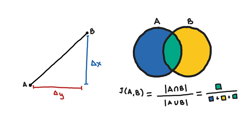
- Cosine Similarity, Euclidean and Manhattan Distance/Norm: Getting the Ln norm or the dot product of a d-dimensional vector takes O(d) time since it requires going through each dimensiom.
- Hamming Distance: If there are d bits, then computation of the hamming distance takes O(d) time. But if you can fit this in a 64-bit number, then you can have an O(1) operation using bitwise operations.
- Jaccard Distance: This involves getting the intersection of two sets. Although doing this using a
setwill be O(m) on average however there can be overhead here that makes it slower than what libraries do. Functions such as numpy.in1d do this by doing sorting the elements of the two sets, O(m log m), and when you have two lists that are sorted, there tricks to get their intersection in linear time. - Edit Distance: Also known as, Levenshtein distance, which is used by libraries such as fuzzywuzzy. The solution to this uses dynamic programming and takes O(m²) time for two strings each with around m characters. This is the most expensive among the distance metrics.
Matrix Operations
For matrix operations, time complexity can be a bit trickier because optimizations to these operations can be done at very low levels, where we design algorithms to be cache-aware. At this level of optimizations, the big O notation can be misleading because we drop the coefficients and we find fine-tuned algorithms that may be asymptotically slower but perform better empirically. This happens for in high-performance libraries such as BLAS and LAPACK which numpy uses under the hood.
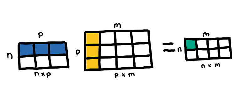
- Matrix multiplication: If you are multiplying two matrices, (n, p) and (p, m) then the general complexity of this is O(nmp), which is O(n³) when multiplying two square matrices of size n. Libraries such as numpy uses BLAS, so the exact implementation of matrix multiplication depends on the BLAS library you are using. See this stackoverflow thread.
- Solving Linear Equations and Matrix Inversion: This runs O(n³) as described in LAPACK benchmarks documentation. I think numpy solves a system of linear equations to also solve the matrix inverse.
- (Truncated) SVD: The classical SVD decomposition is O(nm²) or O(n²m) depending which of n and m is bigger, but if you only need to get the first k dominant eigenvectors, then this can go down to O(nmk)
- Randomized SVD: This is already implemented in sklearn PCA when
svd_solver='randomized'which according to the documentation is O(n²k) but the original paper says O(nm log k) [4]. - Solving Linear Regression using OLS: This is solved in O(nd²) because of the matrix multiplication when solving the hat matrix [6]
Pairwise Distances
This is a simple problem that doesn’t seem to have a simple solution.
If you have a vector v, and you want to get the “nearest” vector in a list of n vectors, then the most straightforward implementation would take O(n) time by comparing v to each n vectors.
More generally, if you have a list of m vectors, and for each vector, you want to get the “nearest” vector in a list of n vectors, this takes O(nm) time. O(n²) if m and n are equal.
If n and m are huge, then this pairwise distances is too slow for a lot of use cases. The solutions that I’ve found so far are the following:
- Spatial index trees: Which can perform O(log n) search on average and O(n) at the worst case. Examples of these are Ball Trees and K-D Trees.
- Random Projections and Locality Sensitive Hashing: This helps us get approximate nearest neighbors with a much faster algorithm.
- NN-Descent: This builds a K-Nearest Neighbors Graph which they have seen to run empirically around O(n^1.14) [5]
Problems with Pairwise Distances

Let’s go further with some use cases that you might encounter and what data structures and tricks are there to help us along the way.
Nearest Point
For geospatial feature engineering, such as geomancer, where for a particular coordinate, we build features by answering questions such as “what is the distance to the nearest ___?”_ and “_how many ____ are within a 1 km radius?”
In both cases, you might naively have to go through all your points, which is O(n). Why? For you to conclude that a point is the “nearest”, you have to have some guarantee that all the other points are further away. For cases where you only have a few thousands of points to search in, this might be acceptable. But what if you want to search in millions of points, or reduce the search time for each query? How do we go about it?
Nearest Point in 1-D
First, we handle the special case where we assume that our points have only one dimension. As a pre-processing step, we sort our array. Let’s say we want to look for the number that is closest to 42. We look at where 42 “fits”, in the example below, this is between 37 and 50. This can be easily done using binary search, O(log n).
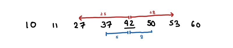 Looking for the number to 42. No point in searching before 37 or after 50.
Notice, that since we know the 42 fits between 37 and 50. We only need to find the closest number in 37 and 50; every point to the left and to the right has to be further than these two points.
Spatial Index Trees
How do we generalize these two 2-dimensions? This is where data structures such as the K-D trees and Ball-trees come in.
A K-D tree maps the space into rectangles, where rectangles that are close in Euclidean space are also close in the tree-space.
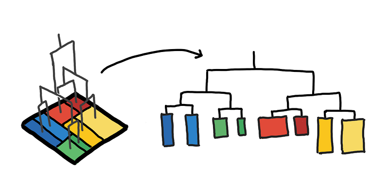 K-D Trees visualized: Mapping a space using a tree
With the K-D Tree we are first able to ask what is the region that contains our query point. This first region has very few points here, probably around O(log n). After getting the distances of all points in this initial region, we get an upper bound for the distance of the nearest point.
 Only visit regions that intersect with the upper bound that we found
We use this upper bound to eliminate neighboring regions that have no choice of containing the nearest point to our query point. Visually, we limit the search space to those regions that intersect with the grey circle.
With this, we are able to eliminate a lot of unnecessary distances that helps us achieve an O(log n) search query on average. We can also do “k-nearest neighbors” and “points within radius” queries.
These are the data structures that are implemented in Nearest Neighbor Searches in PostGIS and you can also read more about it in this Mapbox blog post. You can also read more on Nearest Neighbors — Scikit-learn
Most Similar Document / Near-Duplicate Documents
Other use cases that we have are:
- Looking for a document or word that is most similar to a given word embedding
- Finding near-duplicates in a database of records where records can be considered duplicates if they are “close enough” (less than 3 edit distance)
If we were to just find exact duplicates, this would be easier. Since we can use a set to find these duplicates, but because we are looking for near-duplicates, then we have to find a different approach.
The K-D Tree is good but for other use cases such as those in NLP, it may be less useful. Some problems with K-D Tree and Ball Trees are:
- Does not support cosine distance/similarity
- May not work well for high dimensional data
Remember that K-D Trees run O(log n) on average. However, this is is not guaranteed and is only shown to be true empirically. Its worst case is O(n), which occurs more often in high dimensional data.
To understand, recall the illustration above where we limit the regions we explore to those that intersect with the grey circle. In three dimensions, our regions are cubes, and for more dimensions, we have hypercubes. As we increase the number of dimensions, we increase the number of neighbors that our hypercube region has, which means that our ability to limit the number of regions we have to explore degrades since more and more regions are “close” to every other region.
As the number of dimensions increases, the average running time of a K-D tree for a single query drifts from O(log n) to O(n).
Approximate Nearest Neighbor
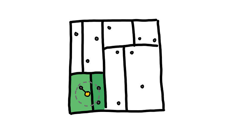
So rather than try to give the nearest neighbor, we can aim to get a nearby neighbor that is “close enough”. One naive way, is to try using the K-D tree, but we skip exploring the neighboring regions and simply search in the region that contains the query point. Or we can also limit to just exploring a set number of neighboring regions. This will guarantee an O(log n), but of course, this affects the overall accuracy.
And if you add a bit more randomness then we got something similar to Spotify’s annoy, which uses random hyperplanes to partition the space instead of just hyperplanes passing through the axes.
](https://cdn-images-1.medium.com/max/800/1*m6b9UHmddhEBxiligpFmyw.png) Random regions partitioned by random hyperplanes by annoy
Random regions partitioned by random hyperplanes by annoy
This approach can be used for distance measures that are not available in K-D trees such as cosine similarity. This is useful for fast lookups for approximately most similar words as described in gensim.
“Brute Force” enumeration
There is a special case when looking for near-duplicate or similar words. For example, doing a search where you want to account for misspellings. The special case is when the query words are short and the maximum edit distance you are willing to tolerate is very small.
In such a case, you can transform the problem into looking for exact matches by enumerating all the possible mutations of your query word.
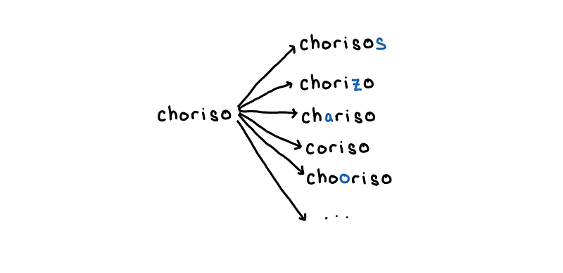 Enumerate all words with edit distance 1 to “choriso”
With word that was enumerated, we simply look this up on our list of words using set . For the example above, the overall cost of this would be the number of possible mutations of the word “choriso” with edit distance at most 1.
for word in enumerate_mutations('choriso', max_edit_distance=1):
   if word in word_set:
       do_something(word)
Quick maths, my rough estimate for the time complexity of this is around O((n52)^k) to enumerate all possible mutations of a word of length n with at most edit distance k. So it is exponential with respect to k.
This is why Elasticsearch’s fuzzy search only allows up to edit distance 2, and why this approach will only work for instances where k is very small, and n is not ridiculously large.
Locality Sensitive Hashing
LSH is a general way of dealing with this problem, and in a way, the annoy package is an implementation of some ideas of LSH.
The general theme of LSH is that we want to limit the elements that we look up to those that are probably similar to our query vector. Let’s say we have the word “chocolate” and want to look for words in our list that are close to “chocolate”.
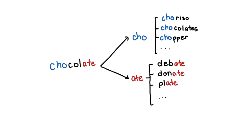 Maybe compare chocolate to words that share the same prefix or suffix
If a word is close to “chocolate” then there is a high probability that they would share the same prefix. Of course, if we limit the words to those that share the same prefix, we might miss out on words that differ only in their prefixes. We can also include words that share the same suffix. So it becomes less likely that a word that is similar to “chocolate” would have a different prefix and suffix.
In this case, our “hashes” for our words are the prefix and suffix, and words with a collision in one of the hashes become candidates for comparison. For vectors, you can use random subsets of columns or random projects for hashing and use MinHashes, which you can read more on Chapter 3 of Mining Massive Datasets [7].
Implementations for python are datasketch, Facebook faiss, and NearPy
If you are interested in more of this you can also look at these blog posts on Big Data using Sketchy Structures, part 1 and part 2.
Clustering Algorithms
In this, we will just go through several clustering techniques and what time complexity we can expect from them.
K-Means
In K-Means, each point is assigned to the centroid that it is closest to. Again, this requires comparing the distance of each centroid to the current point. If there are n points and k centroids, then each iteration takes O(nk). This has a hidden coefficient of the number iterations we expect before the algorithm converges.
If you want to do some hyperparameter search for k by iterating possible values of k, then we expect the overall complexity to be O(nk²).
Mini Batch K-Means
Mini Batch K-means does each iteration over a random sample of the original data set instead of the whole set. This means that we do not have to load the entire data set in memory to do one iteration, and the centroids can start to move to a local optimum as you go through the large data set. This has similar themes that we find in stochastic gradient descent. We expect the overall complexity to now be O(mk), where m is the batch size.
Hierarchical Agglomerative Clustering
You have several flavors for this such as ward, single, complete, and average linkages, but they all have one thing in common, they need to create a distance matrix. This means that classical HAC algorithms are guaranteed to have at least Ω(n²) runtime, and according to the scipy’s documentation, linkage methods run in O(n²) time.
Unless you provide a distance matrix of your own, libraries such as sklearn.cluster.AgglomerativeClustering and scipy.cluster.hierarchy., which sklearn also calls internally, will eventually create a distance matrix using scipy.spatial.distance.pdist .
HDBSCAN
HDBSCAN, which is an iteration of the DBSCAN, is a nice algorithm that clusters the data with a few hyperparameters, no strong assumptions underlying distribution of the data, and is robust to the presence of noise.
At a high level, HDBSCAN tries to estimate the density around points and groups together points in areas with high densities.
For some distance metric m, HDBSCAN has two major steps which are both potentially expensive:
- Computation of core distances: For each point, get the k-nearest neighbors based m.
- Construct a minimum spanning tree: Construct an MST from a fully connected graph, where weights of the edges are based on the core distances and the metric m.
For the general case, both tasks are potentially O(n²) in complexity, which the authors of HDBSCAN try to address in [8]. However, a key detail here is that we are dealing with a distance metric, for example, Euclidean distance, and there are optimizations we can do to speed up both tasks.
The computation of core distances requires k-nearest neighbors, which we have already discussed can be sped up using K-D trees or Ball trees. This means that this step is between O(n log n) and O(n²) on average.
The construction of a minimum spanning tree efficiently is outside the scope of this blog post, but very briefly, the modified Dual Tree Boruvka algorithm uses a space tree such as K-D trees and uses this to find nearest neighbors between connected components. The authors say that this runs on average O(n log n).
With those, then the average run time of HDSCAN would be around O(n log n), but this performance really depends on the data.. The computation of the core distances alone can reach O(n²) depending on the number of dimensions of the data and on the underlying distribution of the data.
Should I get a coffee?
To summarize the different clustering performances, the benchmarking section of the HDBSCAN docs has a neat table that we can use.
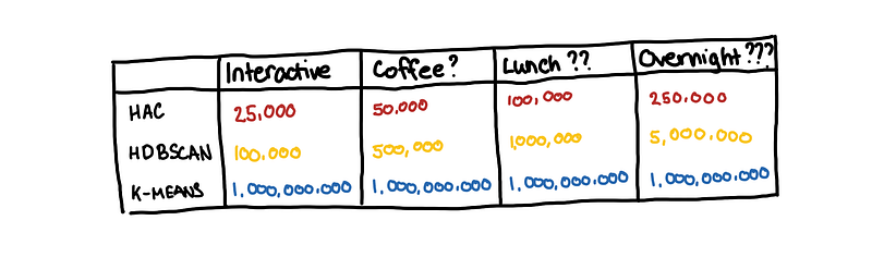 HDBSCAN for 1000000 samples? Let’s get lunch first!
Big Data is hard

As you can see, problems such as getting pairwise distances are very trivial for small data sets but become increasingly problematic as we scale our dataset.
However, if we can exploit certain properties of the problems, such as having a metric distance measure, then we can reduce the running time using data structures K-D trees.
Another approach would be probabilistic algorithms and data structures such as LSH and randomized SVD to get a speedup in run time for reduced accuracy.
Solutions are less clear for problems that are more ad-hoc. That is where a good background on the computational costs of your different algorithms and design choices.
References
[1] Michael I. Jordan. “On computational thinking, inferential thinking and data science”. IST Lecture, Nov 2017.
[2] Andrew Gelman. “N is never large”. July 2005.
[3] Tim Hunter, Hossein Falaki and Joseph Bradley. “Approximate Algorithms in Apache Spark: HyperLogLog and Quantiles”. Databricks Engineering Blog. May 2017.
[4] Halko, Nathan, Per-Gunnar Martinsson, and Joel A. Tropp. “Finding structure with randomness: Probabilistic algorithms for constructing approximate matrix decompositions.” SIAM review 53.2 (2011): 217–288.
[5] Dong, Wei, Charikar Moses, and Kai Li. “Efficient k-nearest neighbor graph construction for generic similarity measures.” Proceedings of the 20th international conference on World wide web. ACM, 2011.
[6] Cho-Jui Hsieh. “STA141C: Big Data & High Performance Statistical Computing”. UC Davis.
[7] Leskovec, Jure, Anand Rajaraman, and Jeffrey David Ullman. Mining of massive datasets. Chapter 3. Cambridge university press, 2014.
[8] McInnes, Leland, and John Healy. “Accelerated hierarchical density clustering.” arXiv preprint arXiv:1705.07321 (2017).
Photos: Pixabay from Pexels, Krivec Ales from Pexels, Guduru Ajay bhargav from Pexels, SplitShire from Pexels, David Geib from Pexels, Pixabay from Pexels